How HydroForecast 10-Day Seasonal works
Updated October 22, 2025
NOTE: We’re in the process of rolling out our latest generation of HydroForecast Seasonal and Annual models. During this transition, some customers may still be using our legacy Seasonal-2 model while others have access to Seasonal-3.
This article describes our process for creating the HydroForecast seasonal model for an individual basin. This model has a 10-day time step and has been implemented to provide forecasts out 12 months into the future.
Using our neural network approach, we train a “base” model across ~470 sites in North America. The goal of this model is to learn general hydrological principles at a variety of basins. This model is driven by historical weather from ECMWF’s ERA5, satellite observations of snow and vegetation from MODIS and VIIRS sensors, drainage characteristics, and snow water equivalent from NSIDC’s SNODAS. Note that this model is not trained on any weather forecast data; only on historical reanalysis from ERA5. In a later step, this allows us to force the model with different weather forecast traces and obtain a realistic and accurate hydrological response.
This base reanalysis model is the starting point for models designed for a specific basin. Using a machine learning technique called transfer learning, we adjust the base model parameters by “tuning” the model to a specific site. This tuned model generally shows improved accuracy across a broad range of metrics. After tuning, the model is very good at understanding the hydrological conditions of the basin (such as snowpack or soil moisture) and it knows how future weather translates into future flows.
To create seasonal forecast traces operationally, we force the model with historical weather patterns. We call this the analog trace approach.
Analog modeling approach
At each forecast issue time, the analog model combines its understanding of the current conditions of the basin with possible weather patterns which come from 39 years (1982-2020) of historical weather from ERA5 reanalysis. Forcing the model with weather patterns of those 39 years clustered around the month and day of the forecast issue date creates 702 scenarios that simulate realistic future flows, 18 for each historical year (18*39 = 702). As an example, for a HydroForecast issued on 2024-01-01, we force the model with 18 traces clustered around 1982-01-01, 18 traces clustered around 1983-01-01, etc, up to 2020-01-01. Our dashboard and API offer access to 40 of those traces which have been selected carefully to maintain the same distribution of total volumes, including the minimum and maximum trace. This method allows a user to interpret the available traces in scenario planning for minimum, maximum, e.g. “worst case,” “best case."
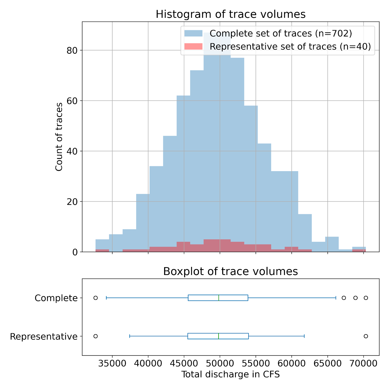
Figure 1: The method selects a representative subset of traces (40 out of the 702) in such a way that the distribution of volumes over the forecast period is maintained between the two sets. The bottom subplot shows the summary of the two distributions in the form of boxplots which are almost identical.
To create our final forecast, we have two strategies that depend on the forecast horizon:
- In the first 30 days, we select a subset of traces that are most likely to materialize- each scenario is selected or rejected based on its “similarity” to the current 35-day weather forecast from NOAA’s Global Ensemble Forecasting System (GEFS). From this subset of traces, we calculate quantiles and the mean.
- For forecast horizons of more than 30 days, we use the full set of 702 traces to calculate the quantiles and the mean.
Accessing the 'Traces' and 'Distribution' views of seasonal forecasts in the dashboard
The “traces” view displays the individual traces and their arithmetic mean. The traces are denoted by an identifier 1-40. Traces with identifier 41-43 are also present through our API but they have empty values. These columns are just a placeholder at the moment and should not be used.
The “distribution” view aggregates traces into quantiles and mean. For analog traces days 1-30, we use the most similar traces to compute the final quantiles and the mean.
In the final post processing step, we replace our seasonal quantiles for days 1-10 with the quantiles forecasted by our short-term model. This is done to take advantage of the better accuracy of our short-term model in those first 10 days. Note that since our short-term model does not produce traces, there can be a disconnect between the trace view (coming from the seasonal model) and the distribution view (coming from the short-term model) in the first 10 days of our forecast.
 Figure 2: Traces view in our dashboard.
Best Practices for Using Seasonal Traces and Distribution Values
- For forecast horizon days 1-10, we recommend using the “distribution” view. In the first 10 days, our distribution comes from the short-term model which has generally better accuracy. We also recommend consulting the short-term forecast section in our dashboard for more short-term information.
- The “trace” view for analyzing traces via our API is particularly useful for aggregating flows over time to obtain seasonal volumes. To create extreme scenarios, aggregate the flows and use the minimum and maximum volumes.
- The “distribution” view or analyzing quantiles via our API is great for getting an accurate picture of the potential flows during any given 10-day period. It is however not suitable for aggregating values over time to get forecasted seasonal volume.
- The mean of the traces will generally be above the median of the traces because flows tend to be right skewed with 0 flow being the lower limit. Use the mean as an unbiased estimate of the forecasted flows. Use the median to get the flow value that will occur with the highest likelihood.